Growing and shrinking
Stephen Broadberry and John Joseph Wallis have written an interesting new paper (pdf). They argue that much of modern economic growth is due to not only a higher trend growth rate, but also due to fewer periods of shrinking.
It’s easy to reproduce some of their results using the nice maddison package.
Get some packages:
library(tidyverse)
library(maddison)
library(scales)
library(lubridate)
library(broom)
library(ggthemes)
Let’s concentrate on some countries with good data coverage, keep only data since 1800 and calculate real GDP growth rates. We also add a column for decades, to be able to look at some statistics for those separately.
df <- maddison %>%
  filter(aggregate == 0,
         iso2c %in% c("DE", "FR", "IT", "JP", "NL", "ES", "SE", "GB", "US",
                             "AU", "DK", "ID", "NO", "GR", "ZA", "BE", "CH", "FI",
                             "PT", "AT", "CA"),
         year >= as.Date("1800-01-01")) %>%
  group_by(iso3c) %>%
  mutate(gr = 100*(gdp_pc - dplyr::lag(gdp_pc, 1)) / dplyr::lag(gdp_pc, 1)) %>%
  ungroup() %>%
  drop_na(gr) %>%
  mutate(decade = paste0((year(year) %/% 10) * 10, "-",
                         (year(year) %/% 10) * 10 + 9))
Define a data frame with annotations for the World Wars:
df_annotate <- tibble(
  xmin = as.Date(c("1914-01-01", "1939-01-01")),
  xmax = as.Date(c("1918-01-01", "1945-01-01")),
  ymin = -Inf, ymax = Inf,
  label = c("WW1", "WW2")
)
Check out data for some countries:
df %>%
  filter(iso2c %in% c("DE", "FR", "IT", "JP", "NL", "ES", "SE", "GB", "US")) %>%
  ggplot() +
  geom_hline(yintercept = 0, size = 0.3, color = "grey80") +
  geom_rect(aes(xmin = xmin, xmax = xmax, ymin = ymin, ymax = ymax),
            data = df_annotate, fill = "grey50", alpha = 0.25) +
  geom_line(aes(year, gr), size = 0.4) +
  facet_wrap(~country, scales = "free_y") +
  ggthemes::theme_tufte(base_family = "Helvetica", ticks = FALSE) +
  labs(x = NULL,
       y = "Percentage points\n",
       title = "Growth rate of real GDP per capita",
       subtitle = "1800-2010")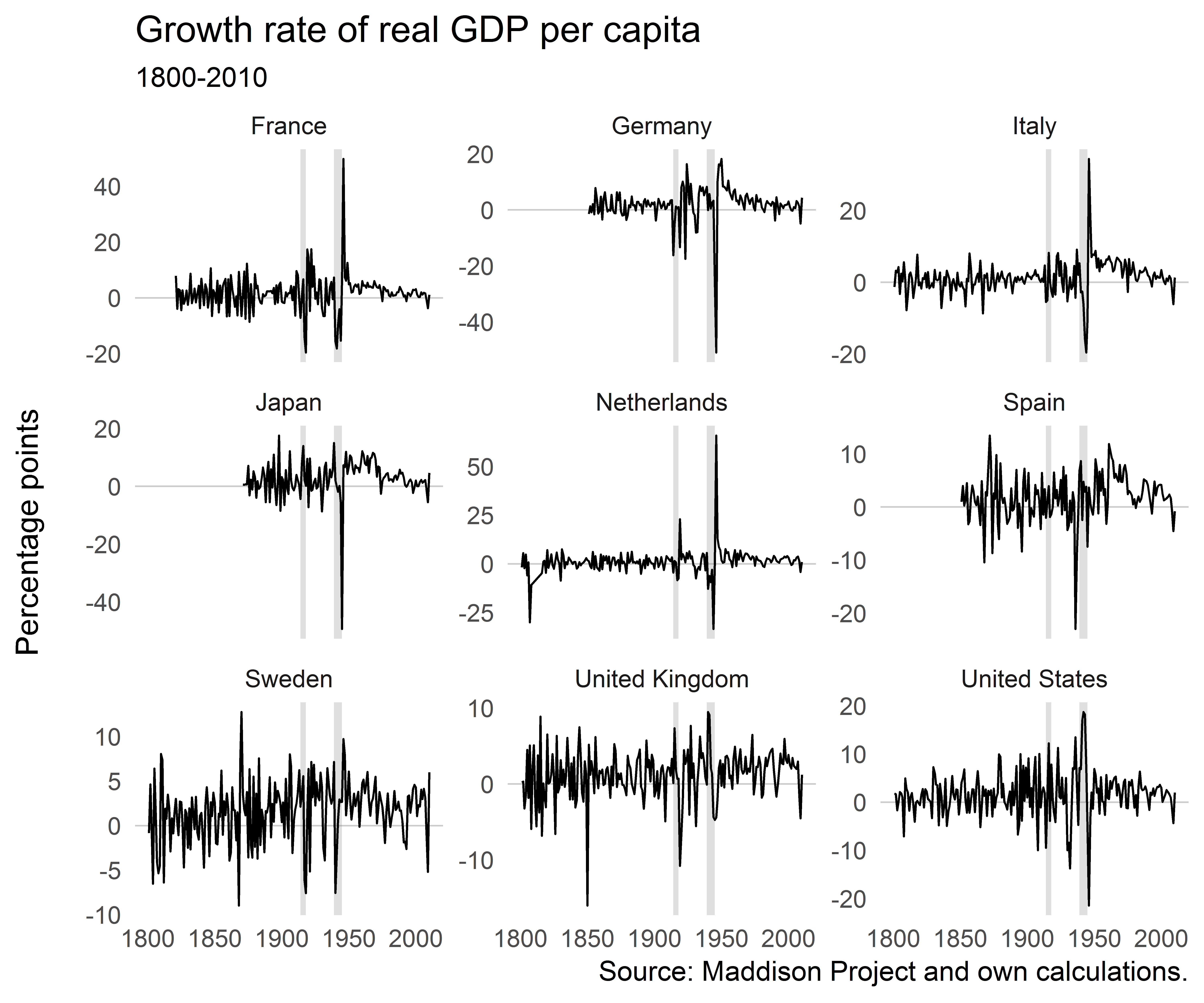
Growth rates wobble around a mean slightly larger than zero, as expected. There are some extreme events around the World Wars. But it’s not immediately apparent from looking at these figures if shrinking has become less. If anything, it’s macroeconomic volatility that has decreased for most of these countries.
Next, for each decade we calculate the number of periods that countries were growing and shrinking and the average growth rates in those periods.
stats <- df %>%
  group_by(iso3c, decade) %>%
  mutate(category = ifelse(gr > 0, "grow", "shrink"),
         gr_av = mean(gr, na.rm = TRUE)) %>%
  group_by(decade, iso3c, country_original, country, category, gr_av) %>%
  summarise(prds = n(),
            delta = mean(gr, na.rm = TRUE)) %>%
  ungroup()

stats <- stats %>%
  left_join(stats %>%
              group_by(iso3c, decade) %>%
              mutate(totper = sum(prds))) %>%
  mutate(frq = prds / totper) %>%
  select(-prds, -totper) %>%
  mutate(comp = frq * delta)
We’re interested in how much growing and shrinking years contributed to overall growth in a decade. So this is just the absolute value of changes by either shrinking and growing years divided by the total variation.
stats <- stats %>%
  full_join(stats %>%
              group_by(decade, iso3c, country_original, country, gr_av) %>%
              summarise(tvar = sum(abs(comp)),
                        gr_comp = sum(comp))) %>%
  mutate(contr = abs(comp) / tvar)
  mutate(dfac = factor(decade)) %>%
  filter(decade != "2010-2019")

ggplot(stats, aes(dfac, comp, color = category,
                  shape = category, fill = category)) +
  geom_hline(yintercept = 0, size = 0.3, color = "grey80") +
  geom_jitter(alpha = 0.5) +
  coord_flip() +
  ggthemes::theme_tufte(base_family = "Helvetica", ticks = FALSE) +
  scale_shape_manual(values = c(17, 25)) +
  scale_colour_manual(values = c("#00BFC4", "#F8766D")) +
  scale_fill_manual(values = c("#00BFC4", "#F8766D")) +
  labs(title = "Contributions of growing and shrinking",
       subtitle = "1800-2009, every point is a country-decade observation",
       y = "Contribution to real GDP growth",
       x = NULL,
       caption = "Source: Maddison Project and own calculations.") +
  scale_x_discrete(limits = rev(levels(stats$dfac)))
When we plot those contributions, we get the following picture:
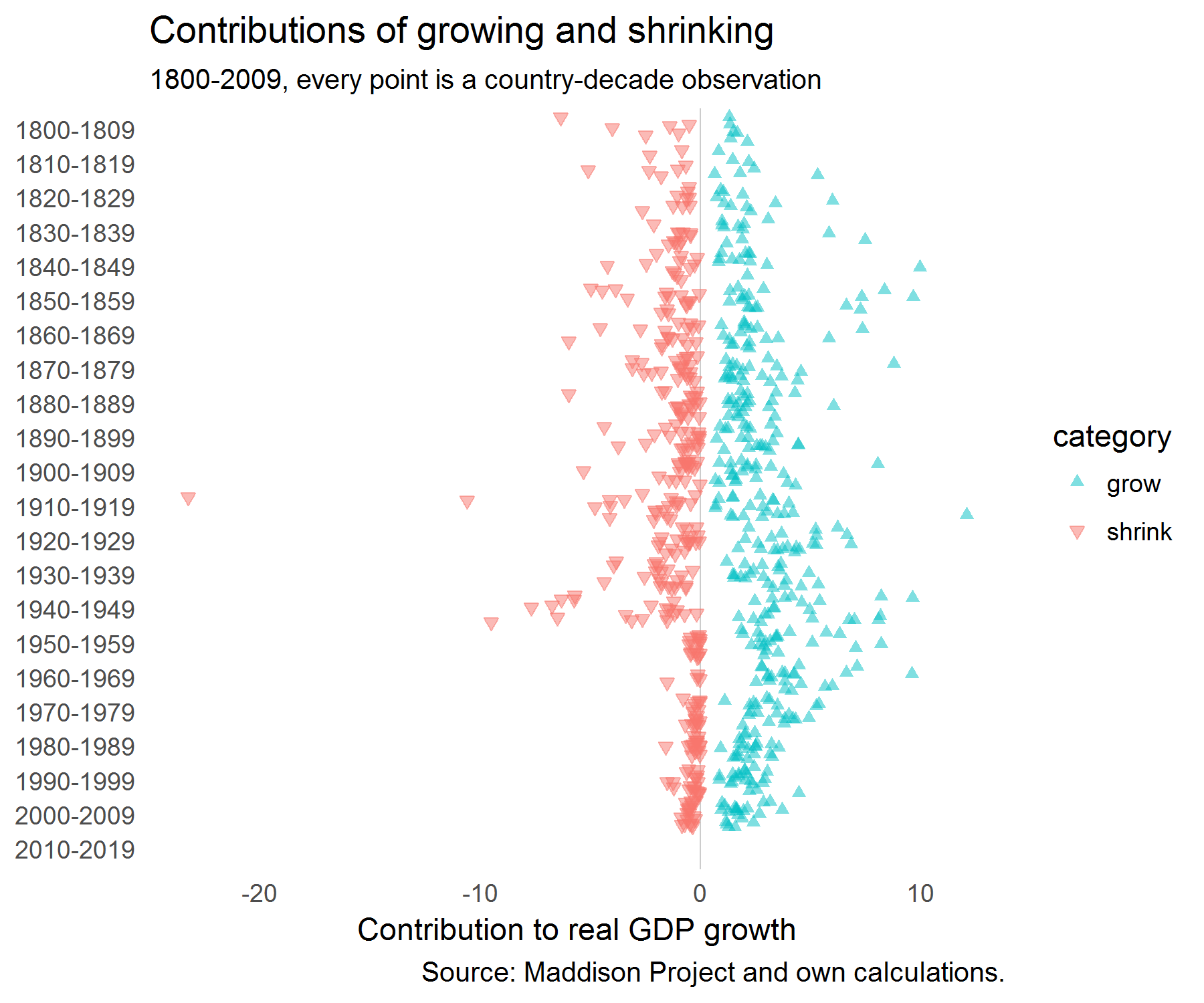
It looks as if the contributions of shrinking have clustered closer to zero since WW2.
Let’s check out the trends in the contribution of shrinking periods:
r <- stats %>%
  mutate(trend = row_number()) %>%
  filter(category == "shrink") %>%
  group_by(iso3c, country_original, country) %>%
  do(fitDecades = lm(contr ~ trend, data = .)) %>%
  tidy(fitDecades, conf.int = TRUE) %>%
  mutate(sig = (p.value < 0.05))
And plot the regression coefficients of the trend line:
r %>%
  filter(term == "trend") %>%
  arrange(estimate) %>%
  ggplot(aes(reorder(country, -estimate), estimate)) +
  geom_hline(yintercept = 0, size = 0.8, color = "grey10", linetype = "dotted") +
  geom_errorbar(aes(ymin = conf.low, ymax = conf.high), width = 0.3) +
  geom_point(aes(y = estimate, fill = sig), shape = 21, size = 1.0, color = "black") +
  coord_flip() +
  theme_tufte(base_family = "Helvetica", ticks = FALSE) +
  labs(title = "Trend of the contribution of shrinking episodes",
       subtitle = "1800-2009 by decades",
       x = NULL,
       y = "OLS estimate and 95% confidence bands",
       caption = "Source: Maddison Project and own calculations.") +
  scale_fill_manual(name = "Significant at 5% level?",
                    labels = c("No", "Yes"),
                    values = c("white", "black")) +
  theme(legend.position="bottom")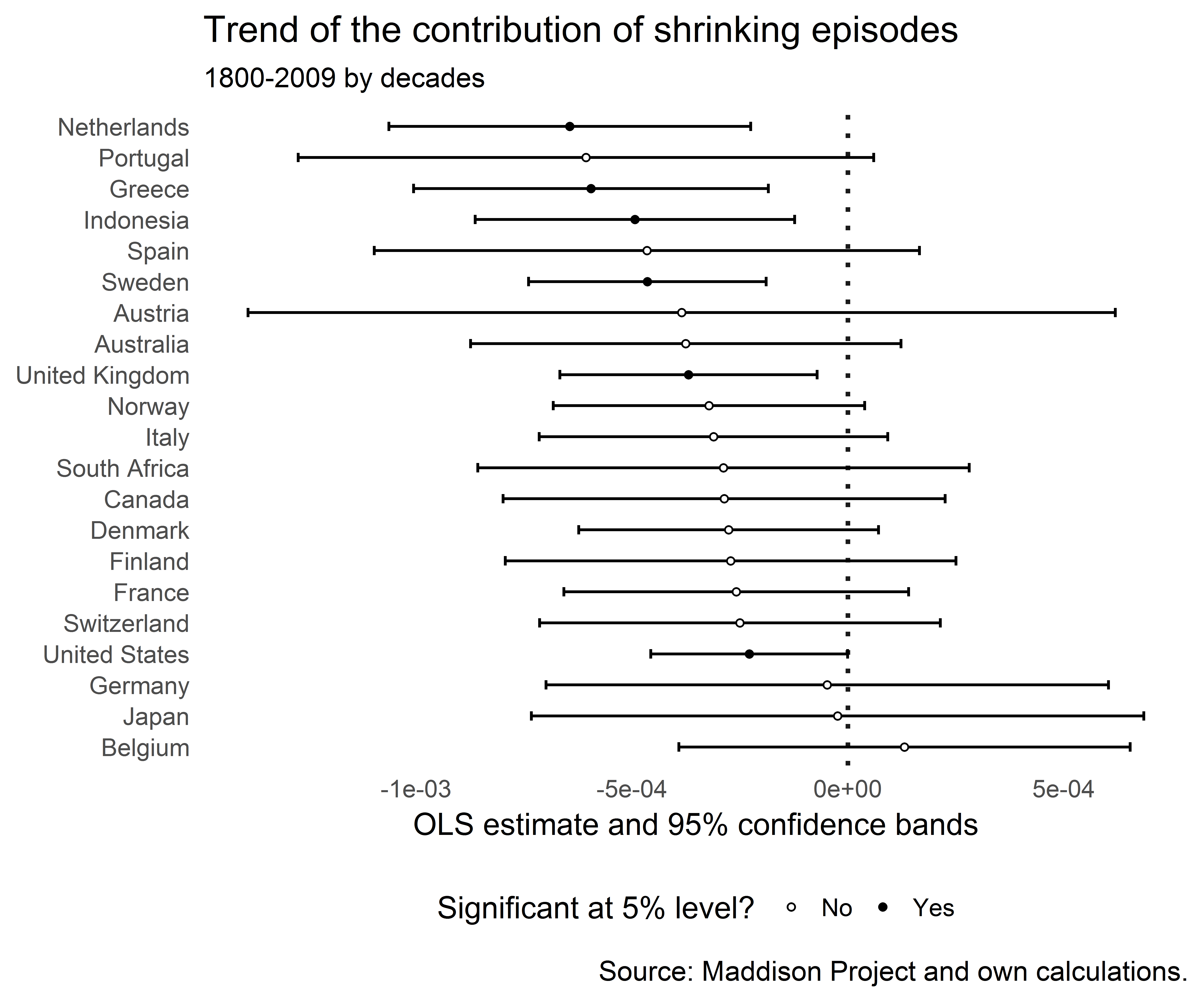
The trend was negative for many countries and for some there was no significant trend. None of the trends was significantly positive. It certainly looks as if episodes of growing output have become more important than episodes of shrinking episodes.
The question remains whether this might not just be mechanically driven by the fact that a higher trend real GDP growth rate reduces the probability of the growth rate hitting zero. And a fall in macroeconomic volatility would also make shrinking episodes less likely.
References
Broadberry, S. and J. J. Wallis (2017). “Growing, Shrinking, and Long Run Economic Performance: Historical Perspectives on Economic Development”, NBER Working Paper No. 23343. doi: 10.3386/w23343