Term spreads and business cycles 3: The view from history
In the first installment in this series, I documented that term spreads tend to fall before recessions. In the second part I looked at monetary policy and showed that it’s the endogenous reaction of monetary policy that investors predict. I worked with post-war data for the US in both parts, but we can extend this analysis across countries and use longer time series.
Start a new analysis and load some packages
library(tidyverse)
library(haven)
library(zoo)
library(lubridate)
library(ggthemes)
library(scales)
library(plm)
library(stargazer)
The dataset by Jordà, Taylor and Schularick (2016) is great and provides annual macroeconomic and financial variables for 17 countries since 1870. We can use the Stata dataset from their website like this:
# Download dataset
mh <- read_dta("http://macrohistory.net/JST/JSTdatasetR2.dta")

# Extract labels
lbls <- tibble(var = names(mh),
               label = vapply(mh, attr, FUN.VALUE = "character",
                              "label", USE.NAMES = FALSE))

# Make tidy "long" dataset and merge with label names
mh <- mh %>%
  gather(var, value, -year, -country, -iso, -ifs) %>%
  left_join(lbls, by = "var") %>%
  select(year, country, iso, ifs, var, label, value) %>%
  mutate(value = ifelse(is.nan(value), NA, value))
Check out the dataset:
mh

# A tibble: 61,200 x 7
# year country   iso     ifs var   label      value
# <dbl> <chr>     <chr> <dbl> <chr> <chr>      <dbl>
#   1 1870. Australia AUS    193. pop   Population 1775.
# 2 1871. Australia AUS    193. pop   Population 1675.
# 3 1872. Australia AUS    193. pop   Population 1722.
# 4 1873. Australia AUS    193. pop   Population 1769.
# 5 1874. Australia AUS    193. pop   Population 1822.
# 6 1875. Australia AUS    193. pop   Population 1874.
# 7 1876. Australia AUS    193. pop   Population 1929.
# 8 1877. Australia AUS    193. pop   Population 1995.
# 9 1878. Australia AUS    193. pop   Population 2062.
# 10 1879. Australia AUS    193. pop   Population 2127.
# ... with 61,190 more rows
Importing Stata datasets with the haven package is pretty neat. In the RStudio environment, the columns even display the original Stata labels.
There are two interest rate series in the data and the documentation explains that most short-term rates are a mix of money market rates, bank lending rates and government bonds. Long-term rates are mostly government bonds.
Homer and Sylla (2005) explain why we usually study safe rates:
The method of using minimum rates to determine interest rate trends is informative. Today the use of „prime rates“ and AAA averages is customary to indicate interest rate trends. There is a very large range of rates higher than minimum rates at all times, and there is no top limit except legal maxima. Averages of rates, if the did exist, might be merely averages of good credits with bad credits. The lowest regularly reported rates, excluding eccentric rates, comprise a practical limit comparable over time. Minimum rates will not show us where most funds were lending, but they should provide a fair index number for measuring long-term interest rate trends. (p.140)
And:
The level of interest rates is a more complex concept than the trend of interest rates. (p.555)
So let’s plot those interest rates:
mh %>%
  filter(var %in% c("stir", "ltrate")) %>%
  ggplot(aes(year, value / 100, color = var)) +
  geom_hline(yintercept = 0, size = 0.3, color = "grey80") +
  geom_line() +
  facet_wrap(~country, scales = "free_y", ncol = 3) +
  theme_tufte(base_family = "Helvetica") +
  scale_y_continuous(labels=percent) +
  labs(y = "Interest rate",
       title = "Long-term and short-term interest rates over the long run",
       subtitle = "1870-2013, nominal rates in percent per year.",
       caption = "Source: macrohistory.net",
       color = "Interest rate:") +
  theme(legend.position = c(0.85, 0.05)) +
  scale_color_manual(labels = c("long-term", "short-term"),
                     values = c("#ef8a62", "#67a9cf"))
Which gets us:
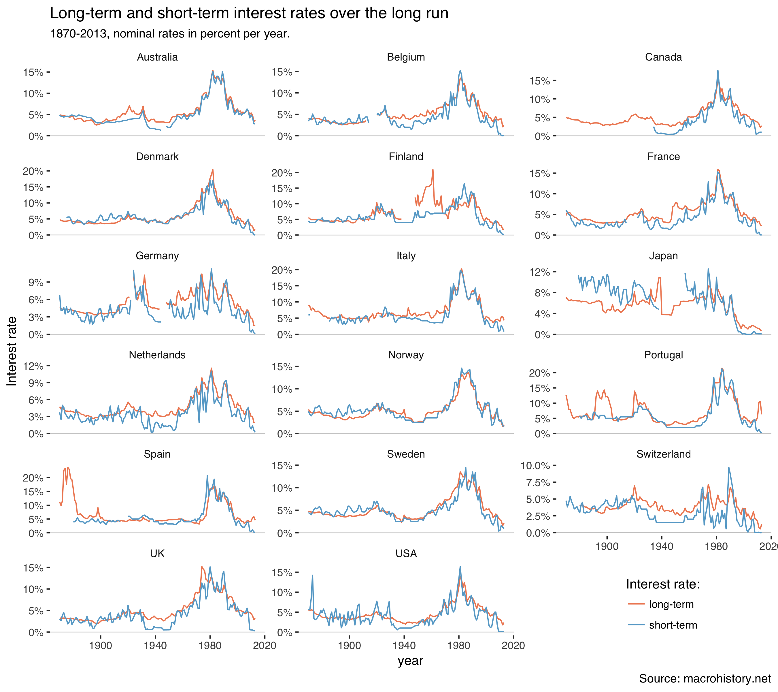
Interest rates were high everywhere during the 1980s when inflation ran high. Rates were quite low in the 19th century. There are also some interesting movements in the 1930s.
Next, select GDP and interest rates, calculate the term spread and lag it:
df <- mh %>%
  select(-label) %>%
  filter(var %in% c("rgdpmad", "stir", "ltrate")) %>%
  spread(var, value) %>%
  mutate(trm_spr = ltrate - stir) %>%
  arrange(country, year) %>%
  mutate(trm_spr_l = dplyr::lag(trm_spr, 1),
         gr_real = 100*(rgdpmad - dplyr::lag(rgdpmad, 1)) / dplyr::lag(rgdpmad, 1))
Add a column of 1, 2, … T for numerical dates:
df <- df %>%
  left_join(tibble(year = min(df$year):max(df$year),
                   numdate = 1:length(min(df$year):max(df$year))))
Check for extreme GDP events (to potentially exclude them):
df <- df %>%
  mutate(outlier_gr_real = ifelse((abs(gr_real) > 15) | (abs(gr_real) < -15),
                                 TRUE, FALSE))
Print the data:
df

# A tibble: 2,448 x 12
# year country iso     ifs ltrate rgdpmad  stir trm_spr trm_spr_l
# <dbl> <chr>   <chr> <dbl>  <dbl>   <dbl> <dbl>   <dbl>     <dbl>
#   1 1870. Austra… AUS    193.   4.91   3273.  4.88  0.0318   NA
# 2 1871. Austra… AUS    193.   4.84   3299.  4.60  0.245     0.0318
# 3 1872. Austra… AUS    193.   4.74   3553.  4.60  0.137     0.245
# 4 1873. Austra… AUS    193.   4.67   3824.  4.40  0.272     0.137
# 5 1874. Austra… AUS    193.   4.65   3835.  4.50  0.153     0.272
# 6 1875. Austra… AUS    193.   4.51   4138.  4.60 -0.0927    0.153
# 7 1876. Austra… AUS    193.   4.57   4007.  4.60 -0.0341   -0.0927
# 8 1877. Austra… AUS    193.   4.39   4036.  4.50 -0.111    -0.0341
# 9 1878. Austra… AUS    193.   4.44   4277.  4.80 -0.357    -0.111
# 10 1879. Austra… AUS    193.   4.60   4205.  4.90 -0.297    -0.357
# ... with 2,438 more rows, and 3 more variables: gr_real <dbl>,
#   numdate <int>, outlier_gr_real <lgl>
Scatter the one-year-before term spread against subsequent real GDP growth:
df %>%
  filter(!outlier_gr_real) %>%
  ggplot(aes(gr_real / 100, trm_spr_l / 100)) +
  geom_hline(yintercept = 0, size = 0.3, color = "grey50") +
  geom_vline(xintercept = 0, size = 0.3, color = "grey50") +
  geom_smooth(method = "lm", size = 0.3, color = "#b2182b", fill = "#fddbc7") +
  geom_jitter(aes(color = numdate), size = 1, alpha = 0.6, stroke = 0,
              show.legend = FALSE) +
  facet_wrap(~country, scales = "free", ncol = 3) +
  theme_tufte(base_family = "Helvetica") +
  scale_y_continuous(labels=percent) +
  scale_x_continuous(labels=percent) +
  labs(title = "Lagged term spread vs. real GDP growth",
       subtitle = "1870-2013, annually.",
       caption = "Source: macrohistory.net",
       x = "Real GDP growth",
       y = "Term spread")
Which creates:
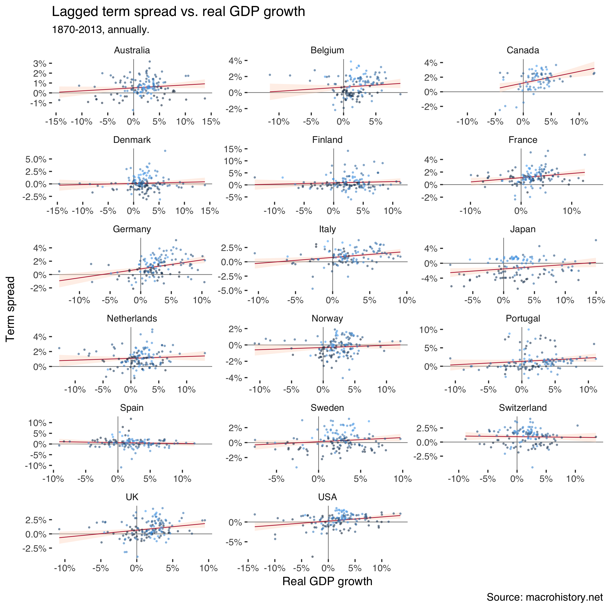
Lighter shades of blue in the markers signal earlier dates. The clouds are quite mixed, so correlations don’t seem to just portray time trends in the variables.
The relationship doesn’t look as clearly positive as in our previous analysis. Let’s dig in further using a panel regression. I estimate two models where the second excludes outliers as defined above. I also control for time and country fixed effects.
r1 <- plm(gr_real ~ trm_spr_l,
          data = df,
          index = c("country", "year"),
          model = "within",
          effect = 'twoways')

r2 <- df %>%
  filter(!outlier_gr_real) %>%
  plm(gr_real ~ trm_spr_l,
      data = .,
      index = c("country", "year"),
      model = "within",
      effect = 'twoways')

stargazer(r1, r2, type = "html")
This produces:
| Dependent variable: | ||
| Real GDP growth | ||
| (1) | (2) | |
| Term spread (lagged) | 0.108* | 0.120** |
| (0.058) | (0.047) | |
| Observations | 2,258 | 2,215 |
| R2 | 0.002 | 0.003 |
| Adjusted R2 | -0.075 | -0.074 |
| F Statistic | 3.474* (df = 1; 2097) | 6.627** (df = 1; 2055) |
| Note: | *p<0.1; **p<0.05; ***p<0.01 | |
So also using this dataset we find that lower term spreads tend to be followed by recessions.
References
Homer, S. and R. Sylla (2005). A History of Interest Rates, Fourth Edition. Wiley Finance.
Jordà, O. M. Schularick and A. M. Taylor (2017). “Macrofinancial History and the New Business Cycle Facts”. NBER Macroeconomics Annual 2016, volume 31, edited by Martin Eichenbaum and Jonathan A. Parker. Chicago: University of Chicago Press. (link)