Inflation: A good sign? — Gourio and Ngo (2016)
I.
Historically, when inflation rose, stock market returns fell. This changed after the financial crisis of 2008. Since then, inflation and stocks have been positively correlated. Why?
François Gourio and Phuong Ngo have written a paper (pdf) in which they address this question. I explore some of their results here, but please go to the source for the full picture.
Stocks are claims to future profits of firms and firms are free to change their prices when the price level changes. So why stocks react at all to inflation has puzzled economists for a long time.
Whatever drove this correlation, it stopped holding after the last financial crisis. The change in the correlation from negative to positive coincided with the US economy hitting the zero lower bound (ZLB) in 2008. The ZLB describes the fact that interest rates are near zero and this leads to many macroeconomic oddities. According to some economic models, positive demand shocks become beneficial at the ZLB, as the inflation they cause reduces real interest rates which leads firms to invest and consumers to buy.
Inflation used to be a sign of a negative supply shock (bad), but now they’re a sign of a positive demand shock (good at the ZLB). And as stocks give you a slice of future expected output of the economy, they react positively to higher inflation at the ZLB.
II.
Start with an agent who receives utility from a stream of consumption:
\[\mathbb{E}_t \sum_{t=0}^{\infty}\beta^t \, \frac{C_t^{1-\gamma} - 1}{1-\gamma}\]where \(\beta \in (0,1)\) is the agent’s patience, \(\gamma > 0\) determines the agent’s risk aversion and \(C_t\) is period \(t\) consumption.
The agent saves in a one-period bond (in zero net supply) with the safe nominal return \(r\) and the agent optimally decides to save and consume according to this Euler equation:
\[\begin{align} \underbrace{c_t^{-\gamma}}_{\substack{\text{Marginal utility of} \\ \text{consumption today}}} &= \underbrace{\beta \cdot (1+r) \cdot \mathbb{E}_t \left ( \frac{c_{t+1}^{-\gamma}}{1+\pi_{t+1}} \right )}_{\substack{\text{Marginal utility of saving} \\ \text{(exp. consumption tomorrow)}}} \nonumber \end{align}\]where \(\pi_{t+1}\) is the uncertain inflation rate. Rearrange and get:
\[\begin{align*} \frac{1}{1+r} &= \beta \cdot \mathbb{E}_t \left ( e^{ -\gamma \, \Delta \, c_{t+1} - \pi_{t+1} } \right ). \end{align*}\]Here we defined \(c_{t} = \ln{C_t}\) and \(\Delta \, c_{t+1} = c_{t+1} - c_{t}\) and used that for small values, \(\ln{(1+\pi_{t+1})} \approx \pi_{t+1}\). Assume that inflation and consumption growth are log-normal, such that \(\Delta \, c_{t+1}\) and \(\pi_{t+1}\) are normally distributed with means \(\mu_{c_t}\), \(\mu_{p,t}\), variances \(\sigma_{c,t}^2\) and \(\sigma_{p,t}^2\) and covariance \(\rho_{t}\).
Applying the rules of the lognormal distribution, we get:
\[\frac{1}{1+r} = \beta \cdot e^{-\gamma \, \mu_{c_t} + \, \frac{\gamma^2}{2}\sigma_{c,t}^2 - \mu_{p,t} + \frac{1}{2}\,\sigma_{p,t}^2 + \gamma \, \rho_{t}}\]Take logs:
\[\ln{(1+r)} = - \ln{\beta} + \gamma \, \mu_{c_t} - \frac{\gamma^2}{2} \sigma_{c,t}^2 + \mu_{p,t} - \frac{1}{2} \, \sigma_{p,t}^2 - \gamma \, \rho_{t}\]The first three terms here mean that rates are higher, the more patient the agent, the higher expected consumption growth and the less risky consumption (as this reduces precautionary savings). The first three terms we would get even if there was no inflation in this model. Call that alternative \(r^{\text{real}}\) and insert it:
\[\begin{align} \ln{(1+r)} &= \ln{(1+r^{\text{real}} )} + \mu_{p,t} - \frac{1}{2} \, \sigma_{p,t}^2 - \gamma \, \rho_{t} \nonumber \\ \underbrace{\ln{(1+r)} - \ln{(1+r^{\text{real}} )}}_{\text{breakeven rate}} &= \mu_{p,t} - \frac{1}{2} \, \sigma_{p,t}^2 - \gamma \, \rho_{t} \label{be} \end{align}\]The breakeven rate is the difference in the returns to a safe nominal and a safe real bond. It increases with expected inflation. But the breakeven rate is not the same as inflation expectations if inflation is uncertain. Instead, it indicates what an agent demands to earn in addition for taking exposure to inflation risk.
The breakeven rate is also greater when inflation and consumption growth are negatively correlated. That is because inflation hurts more when it’s higher at times when consumption is low.1 This markup could even be negative, if \(\rho_t\) is positive – and in combination with \(\gamma\) – high enough to compensate for inflation. Then, the nominal bond becomes a hedge.
III.
This paper now argues that \(\rho_t\) has become more positive at the ZLB.
To argue why, they assume that consumption growth and inflation are driven by a demand and a supply shock. \(\Delta c_{t+1}\) depends positively on both shocks, but \(\pi_{t+1}\) rises with demand shocks and falls with supply shocks.
Assuming independent, zero-mean shocks with constant variances, this means that the covariance between both variables, \(\rho_t\), can be explained by their sensitivity to the shocks and the magnitudes of the shocks. Demand shocks move consumption and inflation in the same direction (higher \(\rho_t\)) but supply shocks work in opposite directions (lower \(\rho_t\)).
Gourio and Ngo offer a neat explanation why there might have been a change in the prevalence of demand and supply shocks: In usual times, the central bank can offset demand shocks, but when at the ZLB it can’t. So the sensitivity of \(\Delta c_{t+1}\) and \(\pi_{t+1}\) to demand shocks might have risen and the sensitivity to supply shocks might even have decreased. This would on net raise the covariance of consumption growth and inflation.
IV.
We can now look at the data and check if the correlation between consumption growth and inflation, \(\rho_t\), became more positive when the economy hit the ZLB in 2008.
The ideal data would be \(\Delta c_{t+1}\) and \(\pi_{t+1}\) from which we could ex post calculate their correlations before and after 2008. Consumption is difficult to measure, so the authors take stock prices instead. These are claims to firms profits and as such to a piece of the aggregate cake. If the savings rate and the profit share of output don’t change too much, then taking stocks (the S&P 500 here) as a proxy for consumption growth might be reasonable.
In principle, we could just use monthly realized inflation for \(\pi_{t+1}\). But due to the short time period, the author’s take the breakeven rate (the difference between the nominal and real 10-year treasury bond yield) as a proxy for inflation expectations.2
Let’s replicate their Figure 1 (codes):
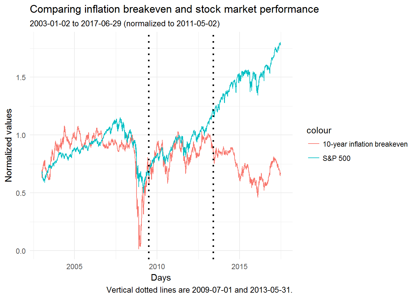
The authors focus on the sample between the two black dotted lines. In that period, inflation expectations and the stock market were firmly positively correlated (ρ = 0.47 ± 0.028).
The story becomes very different after 2013. I wonder why that may be. The Fed Funds Rate was only raised for the first time since the crisis in December 2015. So something else seems to have been driving stocks up and inflation down in the last four years.
References
Coibion, O., Y. Gorodnichenko and D. Koustas (2017). “Consumption Inequality and the Frequency of Purchases”. NBER Working Paper No. 23357.
Fama, E. F. and G. W. Schwert (1977). “Asset returns and inflation”. Journal of Financial Economics, 5(2): 115-146.
Ngo, P and F. Gourio (2016). “Risk Premia at the ZLB: a Macroeconomic Interpretation”. Unpublished manuscript.
-
Somewhat counterintuitively, the breakeven rate also depends negatively on the variance of inflation. The authors explain how this “Jensen adjustment” comes about. I’m still a bit puzzled, because if “higher uncertainty about inflation leads to higher expected payoffs [for the nominal bond]” (p.6), then I’d expect the opposite sign. Maybe the effect is again through precautionary savings. The authors also write: “This term is typically small.” (p.6) ↩
-
That makes the argument strangely circular: We derived formula for the breakeven rate to inform us how \(\rho_t\) matters for the breakeven rate. And now we take the breakeven rate as a proxy for \(\pi_t\). But we’ve just argued that the breakeven rate is not a perfect proxy for inflation expectations, so I don’t quite see how we can do this here. ↩